Flow Matching

[First Draft]

Flow matching gives us a way to model complex real world distributions (target) from simpler or known distrubitions (source).

One way to visualize this is in the form of fluid flow from source to target distributions in \(d\) dimensional Euclidean space, where the fluid is essentially probability mass. We can define a time dependent velocity field in this space which characterizes the flow. Then, converting samples from the source distribution to the target distribution can be thought of as transporting probability mass to convert one density into another along the given velocity field. Therefore our goal would be to learn a suitable velocity field.

For now, let’s limit ourselves to continuous distributions or densities. We can think of the flow to be transporting probability mass over time \(t\), where \(t\) is real and varies from \(t \rightarrow [0,1]\). Let the random variable corresponding to the density at time \(t\) be given by \(X_t\). Let \(p_0\) and \(p_1\) be the source and target densities respectively. Therefore \(X_0 \sim p_0\) and \(X_1 \sim p_1\) are the corresponding random variables. Then, the goal is to convert samples \(X_0 = x_0\) into samples \(X_1 = x_1\).

Animation from Federico Sarrocco’s flow matching blog

Flow and Velocity Field

Let \(u : [0,1] \times R^d \rightarrow R^d\) be the time dependent velocity field. This gives rise to the following ODE :

where \(x\) is a point in \(R^d\). Let \(\psi_t(x)\) be a solution to (1) with initial condition \(\psi_0(x) = x\) :

That is, \(\psi_t(x)\) gives \(x\) at time \(t\) after being transported along the velocity field. This is termed as the flow corresponding to the velocity field \(u\). We will see shortly when such a flow exists and whether it’s unique.

Since we are interested in transporting probability densities, we need to apply the flow \(\psi_t\) to the random variables we’ve defined above, to get random variables and their densities at any time \(t\). This gives us :

Therefore \(\psi_t\) here is transformation on the random variable \(X_0\). Let the density corresponding to \(X_t\) be \(p_t\) :

This is called the pushforward map and is written as :

This can be visualized as below. Let the measure associated with \(p_0\) be \(\mu\) and measure associated with \(p_t\) as a result of \(\psi_t\) be \(\nu\). The probability mass associated with any measurable set \(B\) under the new meausure \(\nu\) must be the same as that of the set \(\psi_t^{-1}B\) under the old measure \(\mu\).

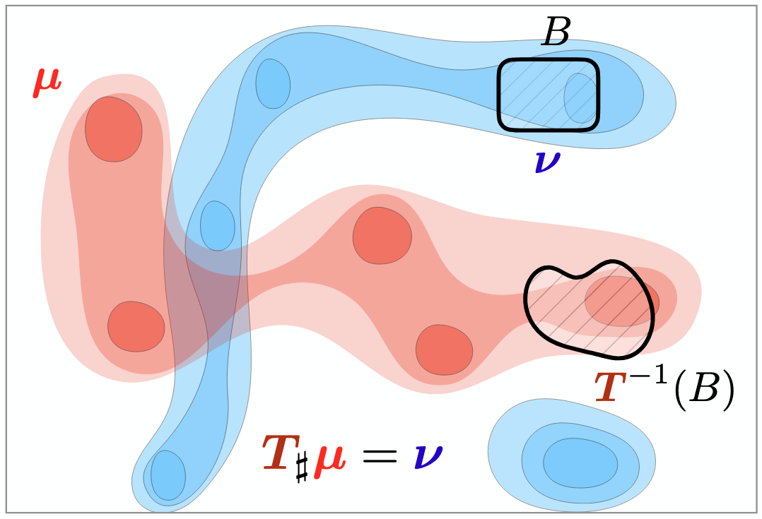
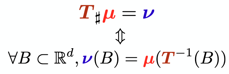
Image from the ICML 2023 Optimal Transport tutorial

As \(t\) varies, \(p_t\) can be thought of as a probability path. It can be shown that if \(\psi_t\) is invertible and differentiable, \(p_t\) can be obtained by the change of variables formula.

Then \(\nu\) is given by :

Therefore :

where \(J\) is the Jacobian. Intuitively, the Jacobian of a function represents how it behaves locally as a linear transformation. The Jacobian determinant then gives us a measure of how much the space is getting ‘streched’ locally. This is the weight on the probability mass that arrived from \(\psi_t^{-1}(x)\). This also means that in order for us to compute (5), \(\psi_t\) has to be invertible, and differentiable. This can be enforced in a principled way in terms of a diffeomorphism.

Let \(C^r(R^m, R^n)\) denote the collection of functions \(f : R^m \rightarrow R^n\) with continuous partial derivates of order \(r\). Then, \(C^r\) diffeomorphism is a class of invertible functions with \(\psi \in C^r(R^d, R^d)\) and \(\psi^{-1} \in C^r(R^d, R^d)\).

We can constrain flows and velocity fields to be \(C^r([0,1] \times R^d, R^d)\) diffeomorphisms. Let’s call this design choice 1.

This constraint also allows us to comment on the existence and uniqueness of solutions \(\psi_t(x)\) to equation (1). From Lipman et al. :

Theorem 1 : (Flow local existence and uniqueness). If \(u\) is \(C^r([0,1] \times R^d, R^d), r \geq 1,\) and locally Lipschitz in \(x\), then ODE (1) has a unique solution which is a \(C^r(\Omega, R^d)\) diffeomorphism \(\psi_t(x),\) defined over an open set \(\Omega\) which is a super-set of \(\{0\} \times R^d\).

A function \(f : R^d \rightarrow R^d\) is Lipschitz continuous if there exists a postive real constant \(K\) such that for all real \(x_1\) and \(x_2\) :

A function is locally Lipschitz continuous if for every \(x\) in \(R^d\) there exists a neighborhood \(U\) of \(x\) such that \(f\) restricted to \(U\) is Lipschitz continuous. In general, Lipschitz continuity is a strong form of uniform continuity for functions which limits the function in terms of how fast it can change. Theorem 1 guarantees only the local existence and uniqueness of a \(C^r\) flow moving each point \(x \in R^d\) by \(\psi_t(x)\) in a limited time frame \(t \in [0, t_x)\).

TODO : what if we allow non-unique solutions? Picard–Lindelöf theorem, Peano theorem, Carathéodory’s existence theorem

To guarantee a solution until \(t = 1\) for all \(x \in R^d\), we must make an additional assumption beyond local Lipschitzness. This is the integrability assumption (design choice 2) :

TODO : Integrability allows assuming that \(X_t\) has bounded expected norm, if \(X_0\) also does.

The mass conservation or pushforward constraint (5) can also be stated in terms of the Continuity Equation :

where \(u_t\) is the time varying velocity field as before, \(x = [x^1, ..., x^d]\) and \(div\) is the divergence operator, given by \(div = \sum_{i=1}^{d}\frac{\partial}{\partial x^i}\). It essentially says that if \(u\) is smooth, given some domain \(D\), accumulating divergences of \(u\) inside \(D\) equals the flux leaving \(D\) by orthogonally crossing its boundary \(\partial D\) (Lipman et al.). If (9) holds, \(u_t\) is said to generate \(p_t\).

In summary, we have defined a velocity field \(u\) and flow \(\psi\) which are both constrained to be \(C^r([0,1] \times R^d, R^d)\) diffeomorphisms. \(u\) is also required to be locally Lipschitz in \(x \in R^d\) and intgrable (in the sense of equation 8) in \(t \in [0,1]\). We have also defined the Continuity Equation (9), which gives us a way to compute \(p_t\) from \(u_t\), and the pushforward constrain (5), which allows us to compute \(p_t\) from \(\psi_t\). And \(\psi_t\) is the unique solution to (1). Therefore if we can learn \(u_t\) we will be able to compute all the quantities.

Given a \(C^r\) flow \(\psi_t\) we can also obtain a unique velocity field \(u_t\) from equation (1) :

where \(\dot{\psi_t} = \frac{d}{dt}\psi_t\).

Towards conditional flows and velocity fields

Flow models can be learned by maximum likelyhood estimation since the log likelyhood \(logp_t(\psi_t(x))\) can be computed for \(t=1\) :

This can be derived from (9) and (2).

TODO : derive

Computing \(div(u_t)\) which is the trace of the Jacobian \(\partial_x u_t(x) \in R^{d \times d}\) is expensive for commonly used \(d\) and requires trace estimators like Hutchinson’s trace estimator. Training requires precisely simulating ODE (10) repeatedly. Flow matching provides a much simpler and more efficient framework that does not involve ODE simulations.

TODO : what do ODE simulations mean in terms of the ‘ground truth’ flow

Instead of ODE simluations, flow matching uses a regression objective for the velocity field using conditional quantities, conditioned on source or target samples. We will see shortly why dealing with conditional quantities is much simpler and more desirable.

Source and target samples can form a joint distribution or coupling, or be independent in which case its called an independent coupling. For example, in case of generating images \(x_1\) from random Gaussian noise vectors, the source and target distributions can be assumed to be independent. For now we can assume independent coupling and later look at other couplings (design choice 3). The probability path \(p_t\) can be computed from conditional probability paths, where the conditioning is on a single sample. Here we assume we can condition on given target samples \(x_1\), but we can also condition on source or jointly on both source and target samples, as we will see later. \(p_t\) is therefore the marginal probability path and is given by :

with boundary conditions (for independent coupling):

where \(\delta_{x_1}\) is the delta measure centered at \(x_1\). The second expression is meant in a limiting sense, since the delta measure does not have a density.

Similarly we can define a conditional velocity field \(u_t(x|x_1)\). From this we can define the marginal velocity as a weighted average of the conditional velocities :

where the weights \(p_t(x|x_1)\) represent the posterior probabilities of \(x_1\) given current sample \(x\). Defining the marginal velocity this way will be further justified shortly when we see that this will imply the mass conservation constraint on the marginal if the constraint is imposed on the conditional. \(p_t(x|x_1)\) can be calculated as :

TODO : interpretation of \(u_t(x)\) as the least-squares approximation to \(u_t(X_t|X_1)\) given \(X_t = x\).

Now we can impose our diffeomorphism, locally Lipschitz, integrability and mass conservation constraints from above, on the conditional quantities. But then we have to verify that given the constraints on the conditionals, the marginals also satisfy them. To satisfy mass conservation, we have to prove the following theorem (Lipman et al.) :

Theorem 2 (Marginalization). Let \(p_t(x|z)\) and \(u_t(x|z)\) be \(C^1([0, 1) \times R^d, R^d)\). Let \(p_z\) have bounded support and \(p_t(x) > 0\) for all \(x \in R^d\) and \(t \in [0, 1)\). Then, if \(u_t(x|z)\) is conditionally integrable and generates \(p_t(x|z)\), \(u_t\) generates \(p_t\) for all \(t \in [0,1)\).

TODO : \(C^1\) instead of \(C^r\)

Here \(z\) is a dummy variable replacing \(x_1\) to denote the fact we could be conditioning on source samples or jointly on source and target samples as well. Conditional integrability is a conditional version of the integrability constraint (8) :

Proof :

This holds from Leibniz’s rule and becasue the assumptions from Theorem 2 make the integrands above integrable. Now if we apply the fact that \(u_t(x|z)\) generates \(p_t(x|z)\) :

from Leibniz’s rule. Multiplying and dividing by \(p_t(x)\) which is positive by assumption :

where the last equality is by (13). We also need to prove that \(u_t\) is integrable in \(t\) and locally Lipschitz in \(x\). \(C^1\) functions are locally Lipschitz and Theorem 2 assumptions imply that \(u_t(x)\) is \(C^1\) for all \(x\). Since \(u_t(x|z)\) is conditionally integrable, by Jensen’s inequality :

TODO : derive

Therefore so far, we have defined a conditional velocity field and probability path. We have also seen that if we impose the necessary constraints on them, that is, if the conditional velocity field generates the conditional probability path, then it also holds for the marginal quantities. This is what we really want, since our goal is to learn \(u_t\). But learning \(u_t\) requires marginalizing over the entire training set, that is, integrating with respect to \(x_1\) in (14). What we need is a loss function with the conditional quantities instead, that still allows us to learn the marginal velocity field.

Loss function

Since we are parameterizing the velocity field, let’s call it \(u_t^\theta\) and the ground truth velocity field \(u_t\) as before. It can be shown that a family of loss functions known as Bregman divergences allows us to learn \(u_t^\theta (x)\) in terms of conditional velocities \(u_t(x|z)\). For now we will use the simplest Bregman divergence which is the Euclidean distance \(D\). Therefore the true loss is given by :

where \(t \sim U[0,1]\) (design choice 4). The conditional loss is given by :

As alluded to above, if \(D\) is a Bregman divergence, we have :

Theorem 3. \(\nabla_\theta L_{FM}(\theta) = \nabla_\theta L_{CFM}(\theta)\)

TODO : Prove

It can be shown (Lipman et al., Liu et al.) that the minimizer of the \(L_{CFM}\) loss in (18) takes the form :

TODO : derive

So, we have defined a loss function that allows us to learn the parameterized velocity from the conditional velocities \(u_t(\cdot|Z)\). However we also do not have access to any ‘ground truth’ \(u_t\), only target samples. We need to be able to define a valid and meaningful \(u_t(\cdot|Z)\) and then regress that onto \(u_t^\theta\).

Optimal Transport

To reiterate, intuitively, we are transporting probability mass from a known source distribution to a target distribution. This can be modeled as an Optimal Transport problem. We can think of the ground truth flow (or velocity field) as an optimal way to do this transportation. We are free to choose what is meant by optimal as long as we are able to justify the choice. Perhaps the simplest choice here is to formulate this as the dynamic Optimal Transport problem with quadratic cost (design choice 5). This results in the ground truth \(u_t\) (and \(p_t\)) which minimizes the kinetic energy :

where the constraint is the Continuity Equation (9). The optimal \((p_t^*, u_t^*)\) can be derived Lipman et al., Villani et al., and gives the flow (using equation (1)) :

where \(\phi : R^d \rightarrow R^d\) is the Optimal Transport map. This formulation gives us straight line trajectories :

Unfortunately we don’t have access to \(\phi\). In fact this is what we want to find in the first place. However our primary goal is to learn a flow that transports probability mass from source to target densities. To this end, we can randomly assign an \(x_1\) to an \(x_0\) and regress the resulting flow (design choice 6). We will explore other alternatives later.

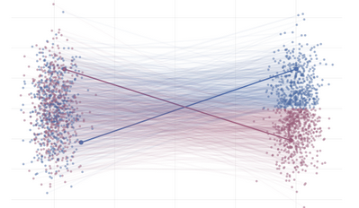
Image from Machine Learning Group, Department of Engineering, Cambridge blog

We can now attempt to find an optimal \(\psi_t(x|x_1)\) (and therefore \(u_t(x|x_1)\)) as follows. From (19) and (20) :

Using Jensen’s inequality :

This gives us a bound on the kinetic energy. Using the tower property of conditional expectations :

Minimizing the integrand in (23) is a variational problem since we are optimizing for \(\psi_t\) :

where the constraints are the result of design choice 6.

This problem can be solved using the Euler-Lagrange equations.

TODO : derive

This gives us the minimizer :

Therefore, the corresponding velocity is given by :

Now we can compute the conditional loss (18) and learn the velocity field. After training, we need to transport a sampled \(x_0\) to the target density. Given our formulation, this can be done easily with the Euler method among others :

where \(h = n^{-1} > 0\) is the step size hyperparameter with \(n \in N\).